
December 2022, Vol. 249, No. 12
Features
Predictive Corrosion Modeling – Rise of the Machines
By Parth Iyer, P.Eng., Mike Westlund, B.Sc., and Wei Liu, M.Sc., Dynamic Risk Assessment Systems, Inc.
(P&GJ) — Pipelines play an important role in the international transportation of natural gas, petroleum products and other energy resources. To ensure pipeline operational safely, instrumented inspections and assessments are completed on a recurring frequency.
One of the most used inspection methods is inline inspection (ILI), a form of nondestructive testing used to assess pipeline conditional integrity. ILI involves using a technologically advanced instrumented tool, propelled within the product flow inside the pipeline, to identify and size corrosion, cracks and other pipe wall defects that can lead to catastrophic structural failure.
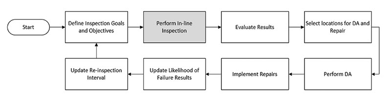
ILI can also record data such as pipe wall loss, pipe geometry deviations in alignment with linear positioning that can be used in the determination of pipeline repair and replacement locations. Figure 1 presents a typical ILI program workflow, based on API 1163 and API 580.
However, not all pipelines are considered “ILI compatible,” and those that cannot be inspected using traditional ILI technologies are typically categorized as difficult-to-inspect (DTI). Challenges to performing an ILI can be categorized into either physical (e.g., design, materials, geometry or location) or operational (e.g., pressure, flow, product or temperature) limitations.
Therefore, the industry typically resorts to alternative assessment methods such as hydrostatic testing or direct assessments (DA) to assess the integrity of DTI pipelines, which can be destructive in nature and may require an interruption in operation.(3) This is the process step in the gray box (“Perform In-line Inspection”) in Figure 1.
In this project, machine learning algorithms were used to predict the location and severity of metal loss corrosion on pipelines, with the intent of providing a nondestructive screening tool that can quickly and reliably aid pipeline operators in assessing the threats of internal and external corrosion on pipelines without ILI data.
Specifically, the algorithm predictions for a specific pipe segment includes a potential for the presence of metal loss (if the metal loss is on the internal or external wall surface) and a regression analysis of metal loss characteristics (corrosion depth, length, width and orientation).
Methodology
This project hypothesizes that a correlation exists between pipeline attributes and operating condition data, and the metal loss reported by ILI. Based on this, machine learning methods are trained to find the correlations and patterns such that accurate predictions can be made when ILI data are not available.
Machine learning methods mainly use statistical methods to train algorithms for classification and regression. Compared with traditional methods, the application of machine learning has the potential to analyze large amounts of data and at a high accuracy level.
Supervised learning, the method used in this project, is the most popular paradigm for machine learning. Based on output variables, a supervised learning method was used for classification (corrosion/non-corrosion, external/internal corrosion) and regression (corrosion depth, corrosion length, corrosion width and corrosion orientation) challenges.
After comparing different supervised learning algorithms, XGBoost1 was chosen for its high prediction accuracy. As one of the most progressive ensemble machine learning methods, XGBoost produces an advanced prediction model in the form of an ensemble of weak prediction models, typically decision trees. Based on the Linux system of VMware and using Python,2,(4) this study implements the XGBClassifier3 and XGBRegressor4 from the Scikit-learn5,(5) module to create the supervised learning classifiers and regressor.
In addition, Grid Search is used to compute the optimum values of hyperparameters when building different models.
Data Preparation
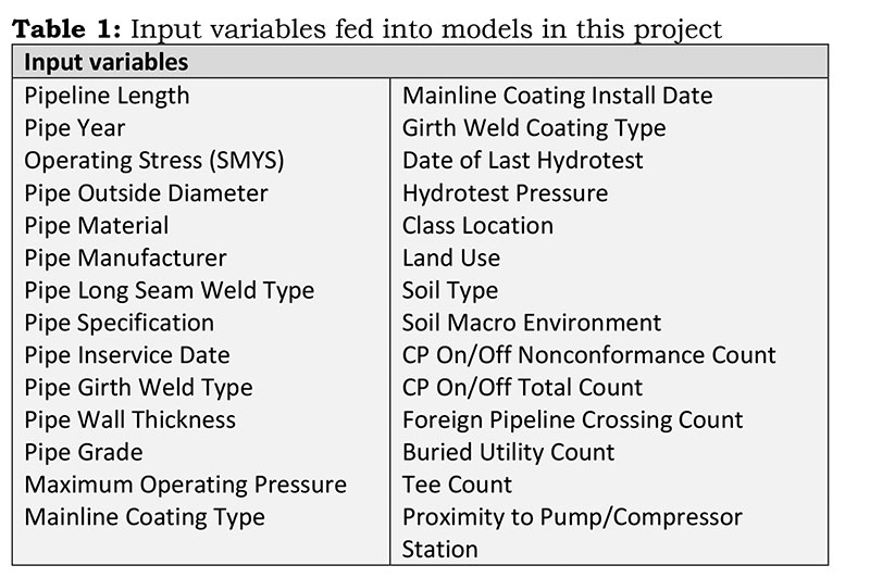
Prior to building the model, data preparation included selecting 28 pipeline parameters, including pipeline attributes and environment conditions as input variables (Table 1). The input variables were selected and extracted from a larger pipeline database used to perform risk assessments, which contains information from multiple anonymized North American pipeline operators.
Data Standardization
Following data preparation, data standardization and consolidation was needed because of the multiple parameters and naming conventions used across pipeline operators within the database. A significant amount of time was spent consolidating the input values to ensure the model would perform optimally.
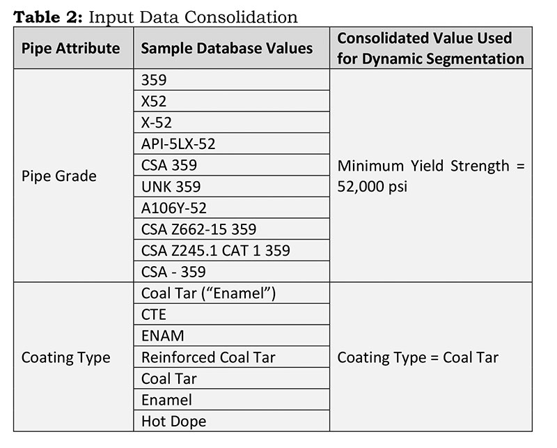
For example, within the data, there were multiple pipe grades and coating types identified that could be consolidated, a subset of which is shown in Table 2. This process was repeated for all 28 input variables to ensure data quality, consistency across the database, and optimal prediction model performance.
Dynamic Segments
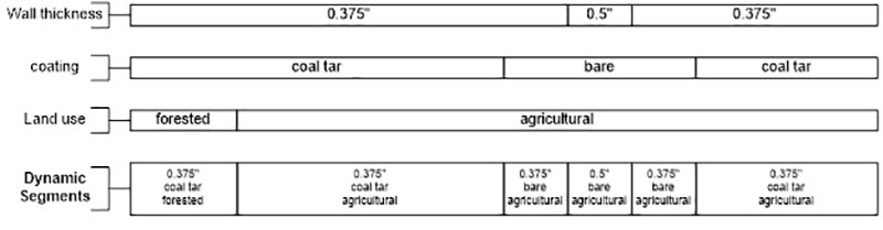
The Dynamic Risk software application makes use of the concept of dynamic segmentation, which is defined as a length of pipe that maintains consistency across specific variables for its entire length. The purpose of this granularization is to establish a discrete length of pipe for each unique set of input variables. Figure 2 provides a simple example of dynamic segmentation in using wall thickness, coating type and land use.
In this example (Figure 2) both wall thickness and coating can be broken up into three discrete linear events, while land use can be broken up into two linear events. Each of these linear events is distinct in their length. When dynamic segments are defined, the linear events can be taken for each variable to create a dynamic segment, of which there are six, each with uniform variable types across its length.
Segmentation for pipelines within the database that have magnetic flux leakage (MFL) ILI was completed based on the 28 linear data attributes (noted in Table 1 and the process outlined in Figure 2). The segments created included the metal loss features from the most recent MFL ILI data for consumption by the predictive model.
Machine Learning
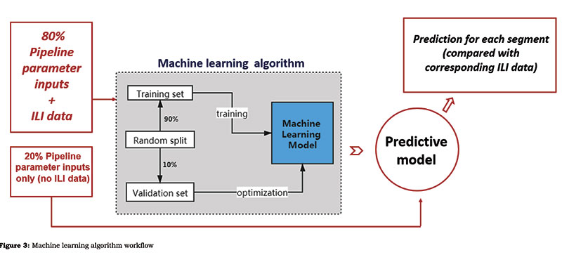
Figure 3 shows the methodology workflow for each prediction model. The database of dynamic pipeline segments was split randomly into a training set containing 80% of the data and a testing set containing 20% of the data. The training set (with the ILI features) was fed into the machine learning model for training and validation so it could identify the patterns within the data.
Upon identifying a correlation between the input features and output labels, the predictive model gained the function to predict the labels of the testing set. The predictive performance of the models was obtained by comparing the predictions with corresponding real data of the testing set.
Model Building
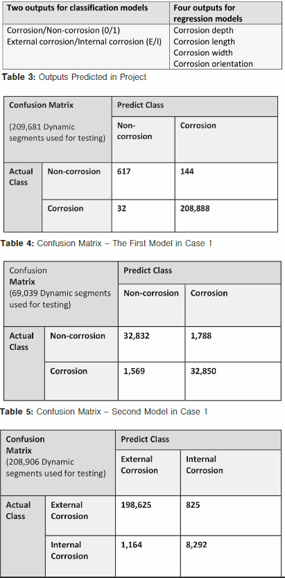
There were six outputs to be predicted, two for the classification model and four for the regression model, as shown in Table 3.
In machine learning, prior to building the model, a set of hyperparameters, defined as parameters whose value is used to control the learning process, need to be identified. The following four hyperparameters were chosen to control the learning process of the models:
- Learning rate: a parameter that helps control overfitting by changing the weight of each new decision tree added to the model.
- Number of estimators: the number of decision trees included in the iterative process of the model.
- Maximum depth: the maximum depth of each individual decision tree.
- Minimum child weight: the minimum sum of weights required to split a node.
To determine the best combination of all hyperparameter values, a function of Python’s Grid Search was used to conduct an exhaustive search of a subset of hyperparameter values. A tenfold cross-validation assessed the performance of each candidate classifier.
In the tenfold cross-validation, a training data set was split into approximately 10 equal size subsets. One subset was chosen as a validation sample and the remaining subsets were used as the training samples. After repeating the training-validation procedure several times, the mean prediction result was compared among all models with different hyperparameter combinations. The model with the best performance was selected to be retained.
In this project, all the models were built by a systematic XGBoost method combining training and validation, hyperparameter selection and model testing. Other supervised learning methods could be used to build this model (e.g., random forest, gradient boosted decision trees); however, the prediction accuracy was found to be lower than XGBoost.
Results
Once trained, the models were introduced to the testing data set. Based on the six different outputs, two classification models and four regression models were built. Results of the classification and regression models are discussed in this section.
Classification Models
Case 1: Corrosion/non-corrosion model
In this case study, the classification model was instructed to predict whether a dynamic segment contained corrosion. Two models were built and compared in this method. In the first model, the best prediction was obtained using 1,048,403 dynamic segments (1,044,527 corrosion and 3,876 non-corrosion).
Only about 20% of these (209,681 samples) were used as part of the test set, which is reflected in Table 4, and the remaining were used to train the algorithm.
Table 4 shows an overall accuracy of 99.92% between the predicted results and the actual results in the first model. The accuracy in corrosion and non-corrosion samples is 99.98% and 81.08%, respectively. A constraint of this model is that the data size of corrosion samples is overwhelmingly larger than non-corrosion samples, which introduces a bias in the training.
To overcome this sample bias, a second model was created by selecting a sample of dynamic segments with approximately equal number of segments having corrosion vs. non-corrosion. This case provided a more complete database and removed any bias by including 172,772 segments with corrosion and 172,422 segments without corrosion.
For the best prediction, a total of 345,194 dynamic segments were used for this second model. Of these, only 20% (69,039 samples) were used as test samples, and the rest were used to train the algorithm. As seen in Table 5, the overall accuracy of the second model is 95.14%.
The accuracy in corrosion and non-corrosion samples is 95.44% and 94.84%, respectively. Even though the accuracy of the second model is slightly lower than the first model, the second model is more reliable and less biased.
Case 2: Corrosion Model
Case Study 2 used dynamic segments that contained ILI corrosion features with the same 28 input variables to predict the surface on which corrosion occurred (external and internal). Two models were also built.
In the first model, the best prediction was obtained from the training and testing using 1,044,527 dynamic segments (997,153 segments with external corrosion and 47,374 segments with internal corrosion). About 20% of these (208,906 dynamic segments) were used as part of the test set, reflected in Table 6.
Table 6 shows an accuracy of 99.05% between the predicted results and the actual results in the first model. The accuracy in external and internal corrosion samples is 99.59% and 87.70%, respectively.
Like Case 1, the challenge in the first model was that the data size of external corrosion samples was overwhelmingly larger than internal corrosion samples. This affected the prediction of the model because of the sample bias. The lower accuracy among the internal corrosion samples can be attributed to fewer training samples and the limitation of input features. Typical susceptibility criteria for internal corrosion such as elevation profile, product composition and coupon data were not available to include in the list of inputs to the model in the project.
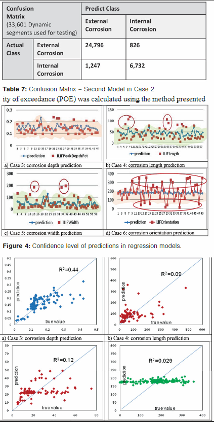
The second model in this case provided a more complete database with less difference between the number of dynamic segments with external and internal corrosion. The database used for this prediction model contained 168,001 dynamic segments that contained ILI corrosion features (128,089 external and 39,912 internal).
Of these, 20% (33,601 dynamic segments) were used as test samples, and the remaining were used to train the algorithm. Table 7 shows that the overall accuracy of this second model is 93.83%. The accuracy for each of external corrosion and internal corrosion samples is 96.78% and 84.37%, respectively.
As with Case 1, the prediction accuracy of the second model using a more complete database is lower than the first model; however, it is more reliable and less bias.
Regression Models
To further predict the attributes of the corrosion within the dynamic segments, four regression models were built in the following four corresponding cases.
Using the same data (168,001 dynamic segments with ILI features) as the second model of Case 2, the corrosion depth (Case 3), corrosion length (Case 4), corrosion width (Case 5), and corrosion orientation (Case 6) are shown in Figure 4.
Confidence Levels
Figure 4 shows a sample of the prediction performance of four regression model cases. Test samples that fall within the shaded region in each of the graphs indicate a 90% confidence in the prediction accuracy.
Nearly all the predicted corrosion depth data are within the 90% confidence area when compared to ILI measured depth. That is to say, the model has 90% confidence to predict the corrosion depth accurately.
For corrosion length and corrosion width, there were some predictions falling outside of the 90% confidence area, which suggest that the models have less than 90% confidence to predict corrosion length and width. In the prediction of corrosion orientation, more than half of the real data fall out of the 90% confidence area, which means the model has weak predictive power for the corrosion orientation.
This low confidence in predicting orientation can be attributed to no input features containing useful information to help the model learn about corrosion orientation.
Correlation Coefficient
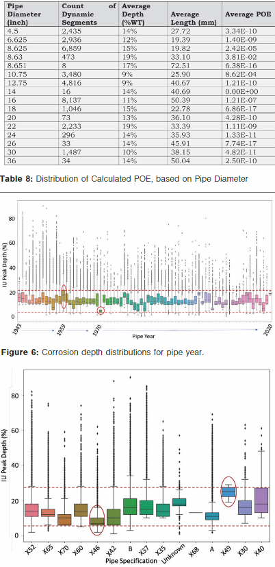
The correlation coefficient (R2) assesses the quality of a model prediction by observing the difference between predicted data and actual data. Figure 5 shows the R2 of the four regression models (Cases 3 through 6).
Results suggest that the model could provide satisfactory prediction of corrosion depth with R2 up to 0.44. The predictive performance of models for corrosion length and width was lower than that of corrosion depth, with 0.09 R2 and 0.12 R2, respectively.
For the corrosion orientation, the model had poor performance of prediction. The R2 was only 0.029 and the prediction values fell into a very limited range (150° to 200°).
Probability of Failure
Typically, for pipelines where ILI data are not available, risk assessment is performed using qualitive models or subject matter expertise.(6) But, with this machine learning approach, a quantitative risk assessment can be performed on DTI pipelines as well.
Therefore, using the depth, length and width prediction, probability of exceedance (POE) was calculated using the method presented by Mihell, et. al (Table 8).(7)
Table 8 shows that NPS 8 pipe on average observed the highest POE values (3.81 × 10⁻²) in the data set. This is because of the larger number of dynamic segments for NPS 8 pipe and the higher predicted depth from the models on NPS 8 pipe. NPS 16 pipe, on the other hand, had the largest sample size in terms of dynamic segments and a very low average predicted depth.
This resulted in a low average POE of 1.21 × 10⁻⁷. NPS 14 pipe was scarcely represented in the database and, because of the shallower anomalies, also resulted in a very low average POE.
Insights
As an output from the database, distributions for each input variable were created to gain more insights on the data and to further analyze the data for trends and commonalities. The figures below show the ILI-measured metal loss depth distributions for two of the input features (pipe year and pipe specification). From the prediction distributions, observations can be made such as the lowest corrosion depths are associated with pipe manufactured in 1970, and the highest ILI metal loss depths are associated with pipe manufactured in 1959 (Figure 6).
The distribution of ILI metal loss features for the input parameter of “Pipe Specification” (Figure 7) indicates that Grade X46 steel is associated with lower ILI-measured metal loss depths.
The highest ILI metal loss depths are associated with a pipe grade of X49; however, after further investigation, the overall population of ILI features in the database that occur in pipe with this grade is very small (accounting for only 10 ILI features). Also, a Grade of X49 is not a typical pipeline grade associated with transmission pipelines.
This input parameter would require further investigation to confirm if the grade of X49 is a unique segment of pipe within the database or a data error. A similar case that would require further investigation exists with the grade of X68, which accounts for only one ILI feature in the database and is likely due to an error in the data.
Distributions can be produced for each of the input variables, such as “Coating Type” and “Pipe Manufacturer,” to gain further insights on the data. Observations made from the distributions then can be used to improve the quality of the input data, validate corrosion risk algorithms, or investigate specific areas of other pipeline segments that contain similar input parameters.
Conclusions
Based on the results obtained from implementing the machine learning model, the following conclusions were made:
Machine learning was used successfully to develop a corrosion prediction model using ILI data and pipeline parameter data.
A significant amount of effort was required to prepare and standardize the data prior to building the prediction model. Depending on the completeness and validity of certain data elements, other variables can be used as proxies for input into the model.
Using a database with equal number of segments (corrosion and non-corrosion) provided slightly lower prediction accuracy. However, the results of this prediction model were more reliable due to lower bias.
Prediction of external metal loss was better than internal metal loss. This result was expected because many of the input parameters catered to external corrosion mechanisms. Input data based on internal corrosion mechanisms were not as abundantly available for this project and may be a consideration for future developments.
In the regression cases, the model could predict the corrosion depth with 90% confidence level and 0.44 R2. Predictions of corrosion length and width were less accurate but considered acceptable. The corrosion orientation could not be predicted accurately because of the limitation of input variables.
NPS 8 pipe showed the highest average POE because of the large sample size and higher average predicted depth.
Output distributions provide data insights for each input variable. Data trends and observations require further investigation and can be useful to improve the data quality or validate actual conditions in other pipeline segments.
This paper demonstrates a proof of concept for a machine learning–based approach to predicting location and dimensions of metal loss. The overall accuracy of the classification models and the high confidence level in the regression models show promise and have the potential, with additional development, to become screening tools for DTI pipelines.
Editor’s note: This paper was presented at the 34th Pipeline Pigging & Integrity Management Conference, Jan. 31- Feb. 4, 2022. © Clarion Technical Conferences and Great Southern Press. Used with permission.
References:
- API RP 580, “Risk-Based Inspection,” Third Edition (Washington, DC: American Petroleum Institute, 2016).
- API STD 1163, “In-line Inspection Systems Qualification Standard,” Third Edition (Washington, DC: American Petroleum Institute, 2021).
- B. Mittelstadt and C. Parker, “Guidelines for Integrity Assessment of Difficult to Inspect Pipelines,” Pipeline Research Council International, 2019.
- G.V. Rossum, “Python,” Python Software Foundation, 1991. Accessed 2021; https://www.python.org/downloads/.
- F. Pedregosa, G. Varoquaux, A. Gramfort, V. Michel, B. Thirion, and O. Grisel, “Scikit-learn: Machine Learning in Python,” J. Mach. Learn. Res. 12 (2011): p. 2825–2830.
- P. Iyer, H. Wu, Y. Nakazato, M. Sen, and L. Krissa, “Estimating the Financial Risk Reductions Associated with Cathodic Protection Programs,” Corrosion 2020 (Houston, TX: NACE, 2020).
- J. Mihell, J. Lemieux, and S. Hasan, “Probability-based Sentencing Criteria for Volumetric In-line Inspection Data,” International Pipeline Conference, 2016.
- A. Rachman and R.C. Ratnayake, “Machine learning approach for risk-based inspection screening assessment,” Reliab. Eng. Syst. Saf. 185 (2019): p. 518–523.
- W.Y. Loh, “Classification and Regression Trees,” WIREs Data Mining and Knowledge Discovery (2011): p. 14-23.

Comments