
July 2023, Vol. 250, No. 7
Features
Sudden Decompression: When the Pressure Gets Released
By Lawrence M. Matta, Stress Engineering Consultant, Stress Engineering Services, Inc.
(P&GJ) — While many integrity management techniques attempt to detect flaws in the early stages, the potential always exists for a defect to initiate a running fracture along the length of a pipe. Cracks can be initiated by, for example, excavation damage, corrosion, or ground movements and may not provide any early warning.
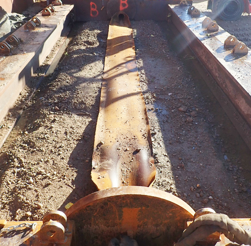
With the wrong combination of pipe material properties and transported fluid, a running fracture may not arrest, leading to a catastrophic failure. Figure 1 shows the results of a running fracture in a test stand that flattened out a section of pipe. Because of this potential, control of fracture propagation is an important part of pipeline integrity management.
It has been known for years that the occurrence of running fractures is determined by a balance between the speed that a decompression wave propagates into the fluid and the speed at which the fracture progresses along the pipe. [1]
If the crack propagates faster than the front of the decompression wave travels through the pipe, then the crack tip always encounters pipe at full pressure. In this case, the crack may propagate until it encounters a valve, crack arrestor, or something else that stops it. At the other extreme, if the fluid decompresses much faster than the crack speed, then the crack quickly encounters unstressed pipe and stops its advance.
If at any point of the decompression the speed of the crack is equal to the local decompression wave propagation speed, there is an opportunity for a running fracture. With the increased transportation of products like CO2 and hydrogen, it is becoming more common to repurpose pipelines and vary the materials transported, and it is worth considering if your pipeline is suited for the new application.
Over the years, there has been a lot of research into fast fracture, and although not all the issues are solved, there are a number of methods and programs available to address it, at least for more typical fluids and pipe materials. For example, API 5L provides four analytical approaches for determining the required CVN absorbed energy values necessary to control ductile fracture propagation in buried onshore gas pipelines (the fifth approach provided is full-scale burst testing). [2]
In addition to other various limitations on their applicability, three of the approaches are recommended for use only for fluids that exhibit single-phase behavior during decompression. In real-world situations, however, many products will encounter a phase boundary during the pressure and temperature drops involved in decompression. This is problematic, because the decompression wave speed typically decreases significantly when the fluid becomes two-phase, allowing the crack to continue progressing. [3]
Subject to other limitations, the Battelle Two-Curve Method (BTCM) is suited for fluids that exhibit single-phase decompression behavior and for rich gases that experience some condensation during rapid depressurization. Application of this method, however, is more complex than the other methods provided by API 5L.
The approach used in the BTCM to characterize decompression is analytical rather than a numerical, Computational Fluid Dynamics (CFD), based approach. To be useful before the age of ubiquitous computers, a semi-analytic expression of decompression speed was developed through its calibration across a variety of gas compositions of common interest. [1] The developed formulation remains useful today, and the BTCM is generally considered as a standard approach for determining required material toughness.
This article explores the decompression process and its behavior. The availability of software such as NIST’s REFPROP [4] provide equations of state that allow for rapid and (in many cases) simple calculation of real gas and phase change behavior on desktop computers. Some examples of interesting decompression calculations using such a tool will be presented, but we will begin with a look into the physics of the decompression process.
Riemann Problems
In the mid-1800s, Bernhardt Riemann considered the problem of how flows develop when a boundary between two fluids with different properties is suddenly removed. This type of scenario is now referred to as a Riemann problem. [5] For a pipeline, the pipe itself can be considered the boundary separating the transported fluid from the outside world, and the boundary can be suddenly removed if the pipe ruptures.
A simple example of a Riemann problem is what’s known as a shock tube, and it can provide valuable insight into how the fluid inside a pipe will behave following a rupture. A shock tube consists of a long, thin tube with a diaphragm located somewhere along its length.
On one side of the diaphragm, the tube initially contains a fluid at a specified pressure and temperature, and the other side of the diaphragm contains a fluid (the same or different composition) at another specified pressure and temperature. The test begins by suddenly rupturing the diaphragm. The pressure immediately begins to equalize, and the fluid on the side with higher pressure expands into the side with lower pressure. Clearly, the behavior of the high pressure fluid bears a similarity to the depressurization of a ruptured transmission pipeline.
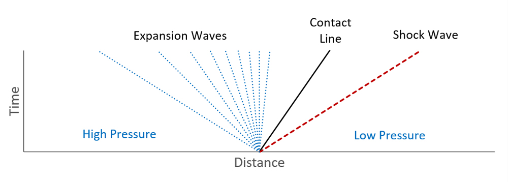
Figure 2 shows a schematic of the development of the flow in a shock tube. At time t = 0, the left side of the tube is at some high pressure, the right side is at a lower pressure, and the sides are separated by a diaphragm boundary preventing the pressure from equalizing. The diaphragm ruptures, and as time progresses, the high-pressure fluid expands and the low-pressure fluid is compressed.
This analysis ignores any mixing (reasonable when the tube is long compared to its diameter), so the two original fluids remain differentiated at a contact line. The solution of the Riemann problem at the contact line is that the pressures and velocities of the two fluids must be equal, while any other property can be different across the contact line.
This makes sense, considering that if they are different fluids, the composition can change across the contact line, but they must flow at the same speed in order to stay in contact but not overlap. The pressure at the contact line will be somewhere between the initial high- and low-pressure.
On the high-pressure side, the front of the pressure disturbance will travel into the compressed fluid at the speed of sound relative to the local flow velocity. The fluid in the shock tube is initially at rest, so the initial disturbance travels at the speed of sound in the undisturbed high-pressure fluid.
Two things occur as the disturbance progresses, 1) the high-pressure fluid expands, and 2) it begins to flow toward the low-pressure end of the tube. Most fluids will cool as they expand (this is not always the case, however), and as they cool, their speed of sound decreases.
This effect causes the wave to thicken into a region of weak expansion waves, as shown by the fan-like appearance of the expansion waves (Figure 1). This thickening effect is enhanced by the increasing velocity of the flow because an expansion wave travels at the local speed of sound minus the velocity of the fluid. If the flow is moving at the speed of sound, an expansion wave cannot propagate upstream through the pipe.
There are two equations whose values are constant across the expansion waves, similarly to the pressure and velocity across the contact wave. These are known as Riemann invariants. Over expansion waves, one invariant is entropy – expansion waves are isentropic. The other condition can be written as:

where u is the flow velocity, ρ is the density, and a is the local speed of sound. These two conditions along with an equation of state (EOS) for the fluid can be used to determine the properties and flow speed through the expansion region. Note that this is the basis for the depressurization equation of the original BTCM, with additional assumptions made to simplify the calculation. Since then, a number of similar methods using various EOS have been developed.
The Riemann problem giving rise to Equation 1 has been solved assuming that the friction takes time to develop a boundary layer across the pipe, and so for a short time after the rupture, the friction can be neglected. Also, heat transfer to the pipe is neglected. Both these become important over a longer distance and duration, but for shock tubes, which can be used as a model of pipelines for a short time following a rupture, testing has shown that these assumptions are reasonable.
On the low-pressure side, a similar process occurs with different results. Similar to the high pressure side, the initial pressure disturbance propagates away from the ruptured diaphragm at the local speed of sound. Because the fluid in front of the pressure disturbance is getting compressed, however, the fluid behind the wave on the low-pressure side is (typically) warmer than the uncompressed gas and has a higher speed of sound.
This increase in the speed of sound means that rather than spreading out, trailing regions of the compression wave continue to catch up to and try to pass the leading edge of the wave. The creates a thin pressure jump known as a shock wave that travels faster than the speed of sound of the low-pressure fluid. Flow through the shock wave is not isentropic.
The property relations across the shock wave are calculated by using a control volume that travels along with the wave, allowing the problem to be analyzed as steady-state. The resulting set of equations are known as the Rankine-Hugoniot equations. Since the shock wave will be on the outside of the ruptured pipe, it is of little use in understanding the pipeline decompression process, and we will not explore the Rankine-Hugoniot equations here.
The pressure and velocity of the contact region will adjust themselves as necessary between the expansion section and the shockwave. Therefore, if there is a need to determine these values, the known conditions in the high- and low-pressure regions must be used to simultaneously solve the expansion and shock relations to find the conditions between the shock and the expansion, which includes the contact line.
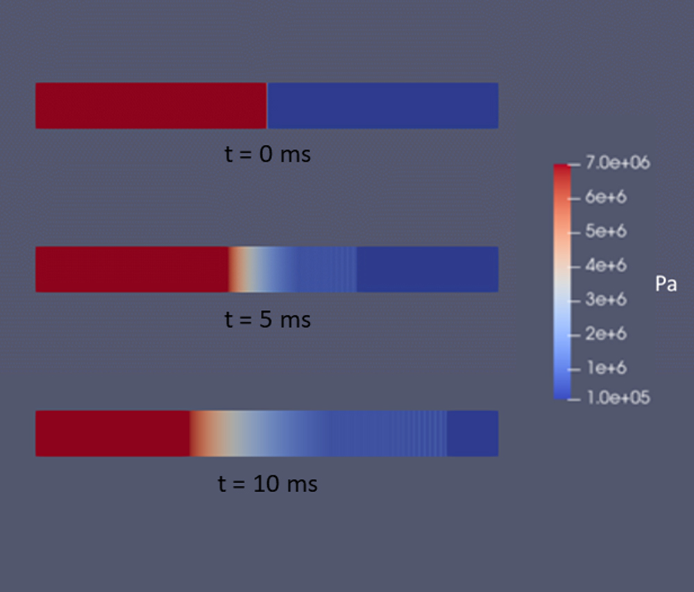
A CFD solution to a shock tube problem (Figure 3). For this example, the fluid is air. The high-pressure side is initially at 1,015 psia (7 MPa) and 70°F (294°K), and the low-pressure side is set to 15 psia (0.1 MPa) at the same temperature. The progression from time t = 0 shows the development of the expansion waves to the left and the shock wave on the right as they move into the undisturbed fluid.
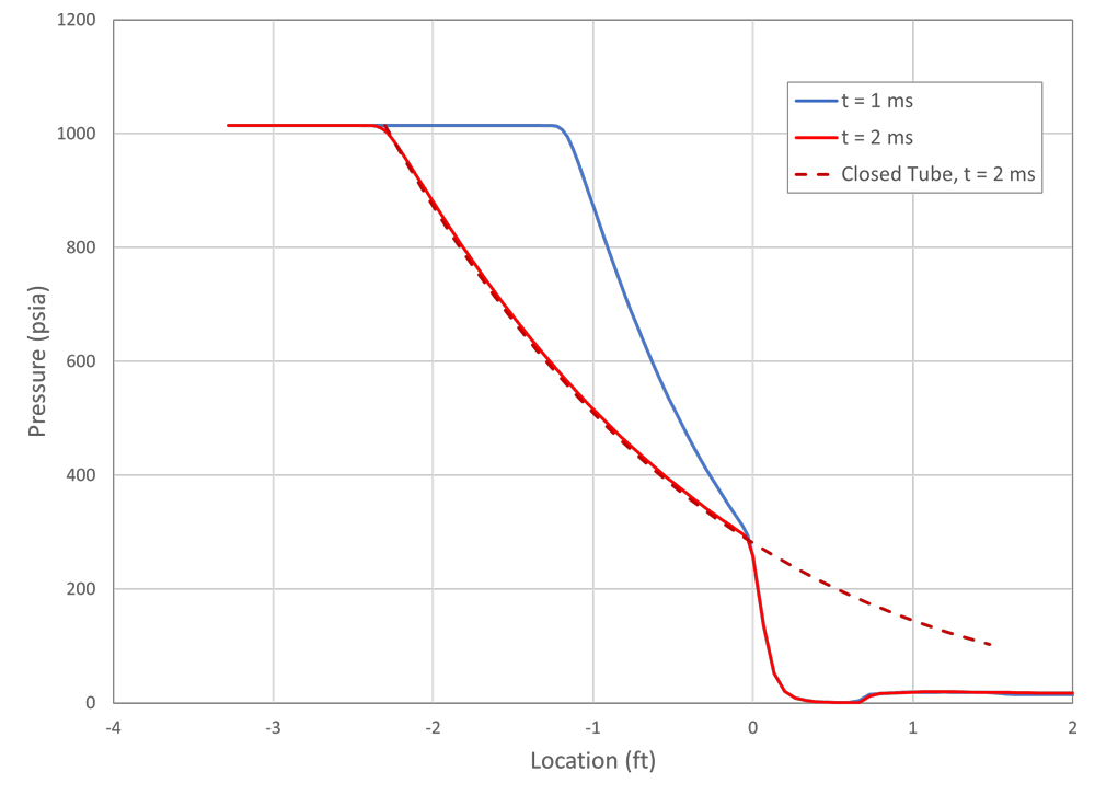
The pressure distributions along the shock tube at two times are shown in Figure 4. Two things are notable from this graph. First is that for air at these initial conditions, the pressure at the contact line is much closer to the low pressure than the high pressure.
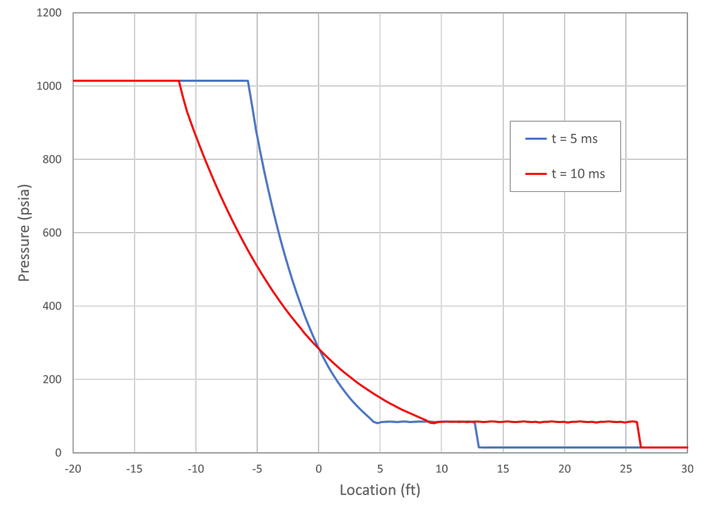
Second, looking at location 0, which corresponds to the initial diaphragm location, the pressure remains constant over time. This occurs when the pressure in the pipeline is above a critical pressure that allows the velocity in the pipe to reach sonic speed.
Generally, any pipeline transporting gas will be operated above the critical pressure, but it is less likely for liquid pipelines. Also, as mentioned previously, this occurs when neglecting the flow friction, and in a long-pipe pressure will not stay constant at the outlet as time increases and the friction becomes the dominant factor in the flow.
Ruptured Pipe
Next, consider one side of a ruptured pipeline. In this case, imagine one side of a full-bore rupture, where the area of the open end is the full cross-sectional area of the pipe. At this point, we will not consider the running fracture, only the fixed location of the rupture. This is conceptually similar to a shock tube in which the diaphragm is at the rupture location.
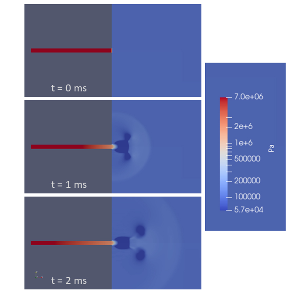
Figure 5 shows results from a CFD analysis of this scenario. The pipe was modeled with the ruptured end at a flat wall open to the atmosphere, so the gray in the figure is solid material. As in the shock tube analysis, the pipe pressure was initially at 1,015 psia (7 MPa) and 70°F (294° K), and the outside atmospheric pressure was set to 15 psia (0.1 MPa) at the same temperature. The end of the pipe was opened at time t = 0. The modeled pipe was round, and the analysis was performed with axial symmetry.
The behavior outside the pipe is complicated, with a roughly hemispherical blast wave (shock wave) progressing away from the rupture location, jet flow from the pipe becoming established, and a smoke-ring-like vortex rolling away from the opening. The flow inside the pipe, however, develops in the same way as the high pressure side of the shock tube. This is demonstrated in Figure 6. In the chart, pressure distributions along the pipe and out into the atmosphere are shown at two times. The corresponding shock tube pressure at 2 ms (labeled “Closed Tube”) is shown for comparison. This shows that the expansion waves inside the pipe are not affected by what happens past the diaphragm/rupture location.
How does the expansion process for a full bure rupture apply to a running fast fracture? As mentioned previously, the expansion waves travel at the local speed of sound minus the velocity of the flow. The speed at which a crack will propagate depends on the pressure in the pipe at the crack tip, among other things.
If the crack can propagate faster than the front of the expansion wave, the crack tip will always see the pipeline at full pressure and the decompression model described previously doesn’t apply to the escaping fluid. If the crack speed is less than the speed of the front of the expansion wave, however, then the expansion region ahead of the crack is not affected by the crack, and the expansion wave solution is valid ahead of the advancing crack tip.
Air, Water
Some insight into the expansion process can be gained by comparing the behavior of air and water. While air is a typical compressible gas, liquid water is often considered incompressible, because under normal conditions a change in pressure results in a relatively small change in density. To compare their behaviors, an expansion wave for each fluid was considered, starting at a pressure of 500 psia (3.4 MPa) and 70°F (294°K). REFPROP was used to perform state calculations. The local pressures as a function of the upstream wave propagation speed (Figure 7).
For air, the decrease in temperature with pressure results in a significant decrease in wave propagation speed. Water, on the other hand, shows a very abrupt change in pressure with propagation speed (in other words, the propagation speed does not change much when the pressure changes). Note that the air is above the critical pressure mentioned above, so the pressure stays elevated at the rupture plane. The water, however, is not above its critical pressure, and so the pressure at the outlet will quickly drop to atmospheric pressure.
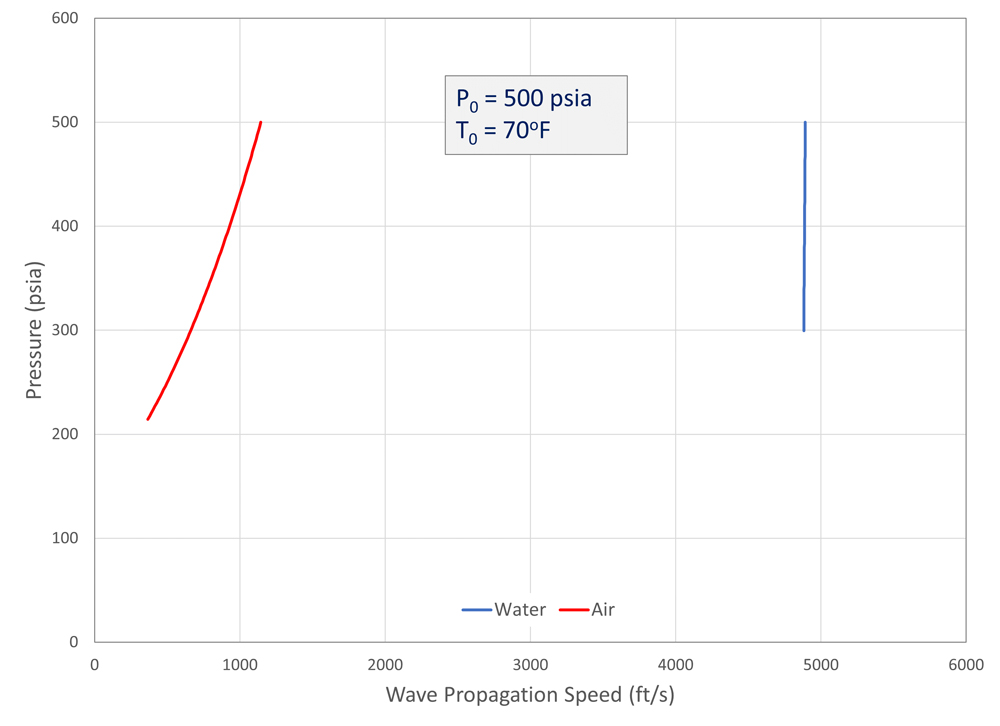
It turns out that the narrow expansion waves in water are not vastly different from the shock waves on the compression side, and this similarity is exploited for water hammer analysis. Also of note is that the wave propagation speed in water is much faster than in air. Fast fracture is much less likely to occur with incompressible liquids than with gases or compressible liquids unless a phase change occurs during decompression.
Before leaving water, it is worth mentioning that because water is not very compressible, the pipe itself can contribute significantly to the wave propagation speed. The change in diameter of the pipe with pressure mimics the effect of fluid compressibility, lowering the wave speed somewhat. This effect was not included in the comparison (Figure 7). For compressible fluids like gases, the effect of pipe wall expansion on the speed of sound is usually negligible.
Carbon Dioxide
The properties of carbon dioxide (CO2) can make it challenging from a fracture propagation standpoint. Consider repurposing a natural gas or oil pipeline to transport CO2. Its liquid-vapor critical point, the temperature and pressure at which there is no longer a distinction between liquid and gas phases, is 1,070 psia (7.38 MPa) and 88° F (304° K).
Natural gas transmission pipelines typically operate at less than 1,100 psia. At ambient temperatures, CO2 can be close to the critical temperature. Thermodynamic properties change rapidly near the critical point. It is also likely that the phase boundary will be encountered during a decompression event. Another issue is that as a liquid at typical ambient temperatures and compressed to 1000 psig, it is quite compressible, with a speed of sound more like that of air than water.
To avoid operation near the critical point, pipelines designed for CO2 typically operate at much higher pressures, but this is likely not possible with a repurposed natural gas pipeline. If the MOP is to low, then a repurposed pipe can only transmit CO2 as a gas, which is less efficient but safer from a fast fracture perspective. The decompression characteristics of CO2 mean that fracture propagation control requires careful consideration. [6]
The issue with phase change is that the speed-of-sound is often significantly lower in two-phase flow than for a single phase. A small volume fraction of mist in a vapor or bubbles in a liquid can significantly affect the wave propagation speed. The reduced wave speed increases the likelihood that a fracture can keep up with the decompression front.
Determining the wave speed is also more difficult because calculation of the sound velocity in two-phase flows is still matter of research. [7, 8] A number of different models exist with different assumptions. In this analysis, the phases are considered to be homogeneously distributed and in thermodynamic equilibrium (temperature and phase), so that the local speed of sound can be calculated as:

where p is the current local pressure and s is the total entropy of both phases.
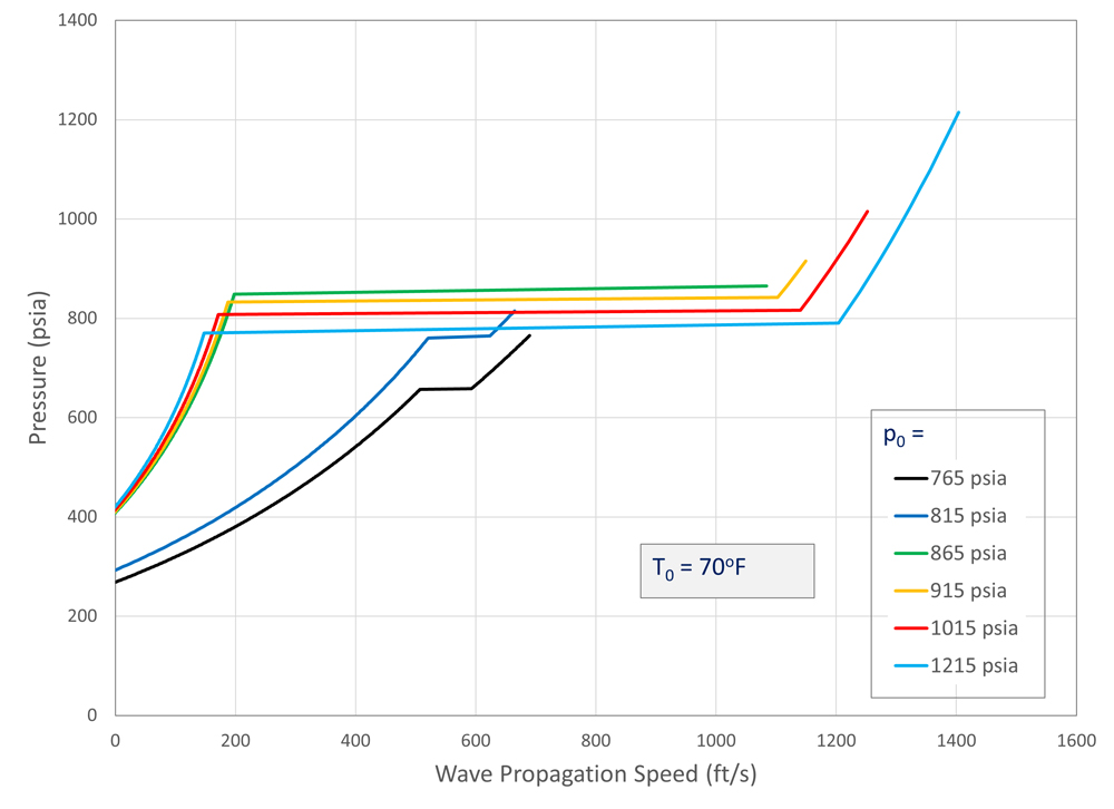
Using this method, Figure 8 shows the decompression behavior for CO2 starting at 70°F (294°K) for a range of pipeline pressures. At 70°F, the boiling pressure of CO2 is approximately 853 psia (5.9 MPa), so the CO2 in the pipeline begins as vapor at pressures lower than this and as a liquid for pressure above this point. The horizontal portions of the curves occur at the saturation line.
The pressure and density are continuous across the saturation line, but the slope changes abruptly, so Equation 2 predicts a jump in the speed of sound. The results show that for this temperature, the worst-case combination of low decompression wave speed with a high residual pressure occurs for liquid flows at pressures just above the boiling pressure. Increasing the starting pressure, however, does not significantly decrease the plateau pressure.
Natural Gas, Hydrogen
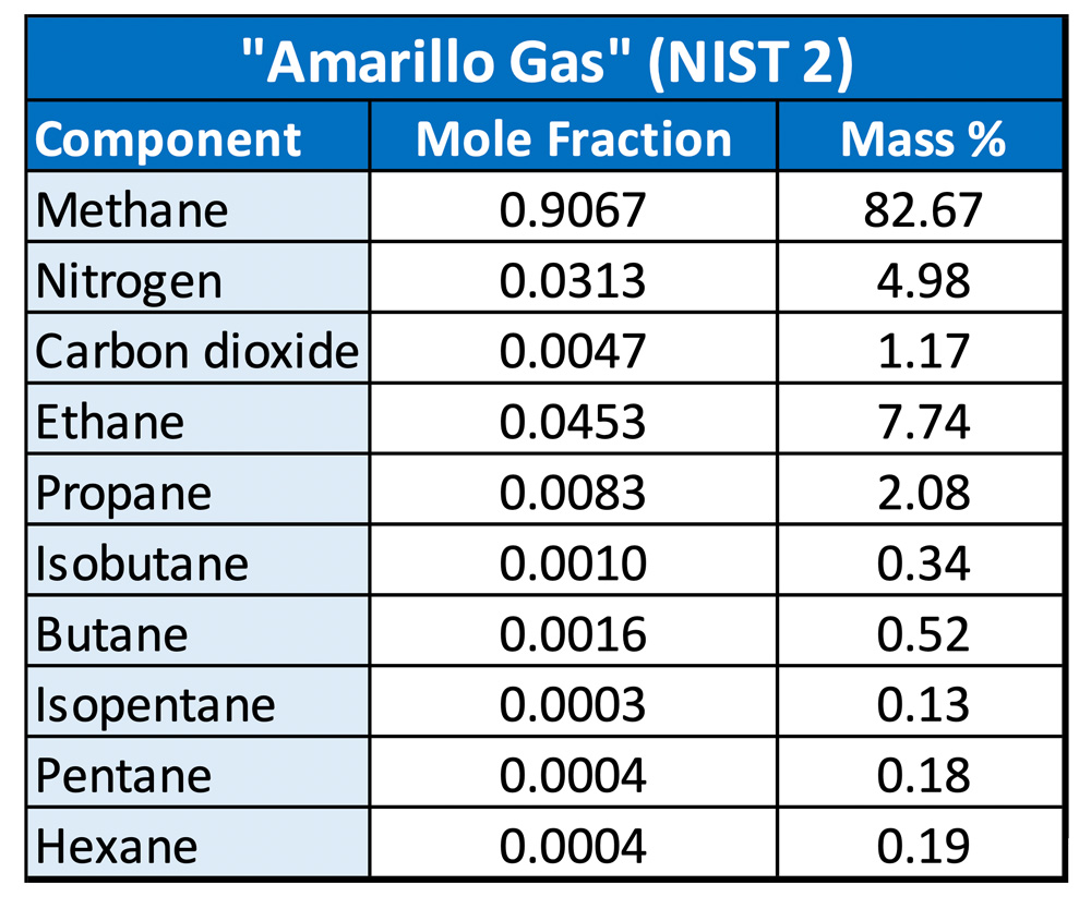
Next, we’ll examine the decompression behavior of natural gas, hydrogen, and mixtures of the two. For this analysis, the “Amarillo Gas” (NIST2) that is included as a pre-defined mixture in REFPROP was used as an example gas. The composition is shown in Table 1.
Natural gas mixtures are considered “lean” or “rich,” based on the ratio of methane to higher hydrocarbons, which also affects their heating values. While there is no strict definition, the Amarillo Gas is somewhere between the two. Lean gases, closer to pure methane, are less likely to produce condensate during depressurization. In rich gases, the heavier hydrocarbons can condense out as the temperature drops.
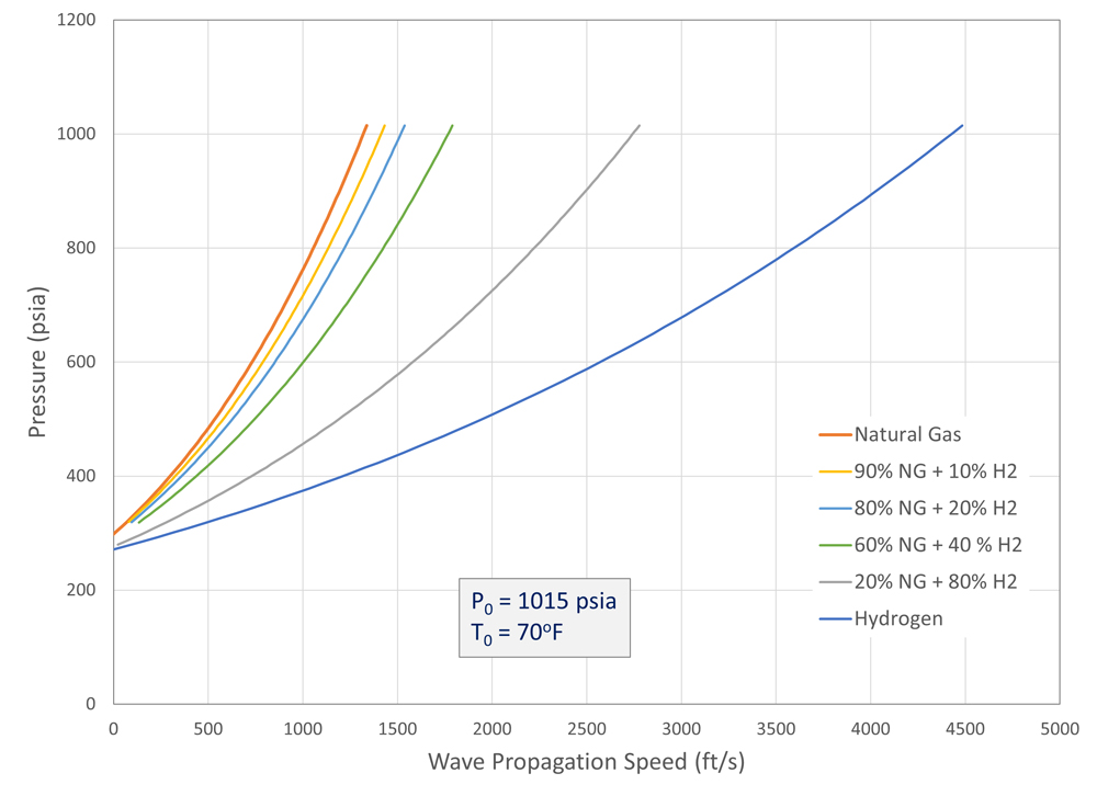
In this example, the pipe pressure was initially at 1,015 psia (7 MPa) and 70° F (294° K), and the pipe opens to atmospheric pressure. From this initial temperature and pressure, the natural gas mix crosses the saturation line as it depressurizes, but the quality stays above 98% and no sudden changes occur in Equation 2 as condensation begins.
The results (Figure 9) show that adding hydrogen to the gas mixture increase the decompression wave speed. The effect is non-linear, so small amounts of hydrogen added to the gas do not significantly affect the decompression wave speed.
A mixture with only 20% natural gas and 80% hydrogen was calculated to have a decompression wave speed roughly halfway between pure natural gas and pure hydrogen. Of course, the result depends on the actual natural gas composition and the pipeline operating pressure and temperature.
Testing and analysis have shown that for some rich natural gases, a plateau region can occur when the dewpoint is reached, and that the addition of hydrogen can increase the pressure of the plateau, increasing the risk of running fracture. [9] The reported tests in which a plateau was observed, however, were performed with an initial pressure of 3,095 psia (21.3 MPa), which is above typical transmission pipeline pressures.
Conclusion
Preventing running fractures is an important consideration in pipeline design and integrity management. It requires ensuring that a crack will not progress along a pipe faster than the pipe will decompress. A number of methods are available to estimate both the fracture speed and the decompression speed as a function of pipe pressure.
This article provided a brief introduction into the physics of the decompression process and some examples of its behavior for pipelines. The analysis for running cracks is concerned with a short time frame – less than a second is typically important. In this timeframe, the flow resembles a shock tube. For a full blowdown analysis, friction and heat transfer quickly dominate the behavior, requiring different analysis methods.
Author: Lawrence Matta, PhD, PE, CFEI is a staff consultant at Stress Engineering Services in Houston, Texas, and applies experience in fluid and solid mechanics, thermodynamics, and combustion to midstream projects. His work includes assisting clients with unsteady flow issues such as pulsation and hydraulic shock induced vibrations.
References:
- Leis, Brian N. et al. “Modeling Running Fracture in Pipelines–Past, Present, and Plausible Future Directions” ICF11 8 (2005): 5759–5764.
- API SPEC 5L:2018-04, ‘Specification for Line Pipe – 46th Edition’, American Petroleum Institute, 220 L Street, NW, Washington, DC 20005-4070, USA (2018)
- Aursand, Eskil et al. “CO2 pipeline integrity: A coupled fluid-structure model using a reference equation of state for CO2.” Energy Procedia 37 (2013): 3113-3122.
- Lemmon, E.W., Bell, I.H., Huber, M.L., McLinden, M.O. NIST Standard Reference Database 23: Reference Fluid Thermodynamic and Transport Properties-REFPROP, Version 10.0, National Institute of Standards and Technology, Standard Reference Data Program, Gaithersburg, 2018.
- D.S. Balsara, Numerical PDE techniques for scientists and engineers (text online) (2013).
- Cosham A., Eiber RJ. “Fracture propagation of CO2 pipelines” Energy. 2003; (049): 115-124.
- Dall'Acqua, Davide et al. “A new tool for modelling the decompression behaviour of CO2 with impurities using the Peng-Robinson equation of state.” Applied Energy 206 (2017): 1432-1445.
- Elshahomi, Alhoush et al. “Decompression wave speed in CO2 mixtures: CFD modelling with the GERG-2008 equation of state.” Applied Energy 140 (2015): 20-32.
- Liu, Bin et al. “Decompression of hydrogen—natural gas mixtures in high-pressure pipelines: CFD modeling using different equations of state.” International Journal of Hydrogen Energy (2019): 7428-7433.

Comments